
The log analyzer loads one or more data logs and plots their channels over time, so you can see what the engine was actually doing. Open it from Analysis › Log Analyzer. This page covers the analyzer window itself; getting a log in is on importing logs, and playing a log back over your maps is on replaying logs over your maps.

The toolbar across the top holds the window’s actions:
.csv, .tsv, .txt, .msl or .log); the import wizard handles the parsing.Two checkboxes, Overlay all logs and Align starts, control how multiple logs are shown (below).
You can load more than one log at a time. The Loaded logs list shows them all; the one you select is the active log, and it drives the channel table and the statistics. Two checkboxes change how they plot together:
The Channels (active log) table lists the active log’s channels in five columns: Show (a checkbox to plot it or not), Color (double-click the swatch to change the line colour), Name, Unit and Group. Channels assigned to the same group (double-click the Group cell to set it) share one Y axis and scale, so related signals sit together and unrelated ones do not fight over a single scale. The channel that is the X axis is marked and cannot be hidden. On import the editor auto-enables the “common four” — RPM, MAP, TPS and AFR — when it recognises them.
The plot is a multi-axis time-series chart. Each group gets its own Y axis, stacked outward from the chart (the first group on the left, the next on the right, and so on), while the X axis — usually time — is shared by all of them. To move around: drag left/right to pan, scroll the mouse wheel to zoom around the cursor, and use Reset View to fit everything again. A crosshair readout follows the pointer, and very dense logs are automatically thinned to what the screen can show so the chart stays responsive without losing its shape.
The Statistics (visible range) panel reports each visible channel’s Min, Max, Mean, Stddev and sample count (N), with its Unit. The figures are computed over the part of the log currently on screen, so zooming into a single pull or a steady cruise gives you the statistics for just that span.
Tip — put related channels in the same group so they share a sensible scale, and keep unrelated ones (say RPM and AFR) in separate groups so neither gets flattened. Then zoom to the section you care about and read the statistics for exactly that range.
All-in-one application for tuning experts preparing vehicles for track use. Designed for professional workshops, it simplifies the deactivation of non essential components to unlock true performance.
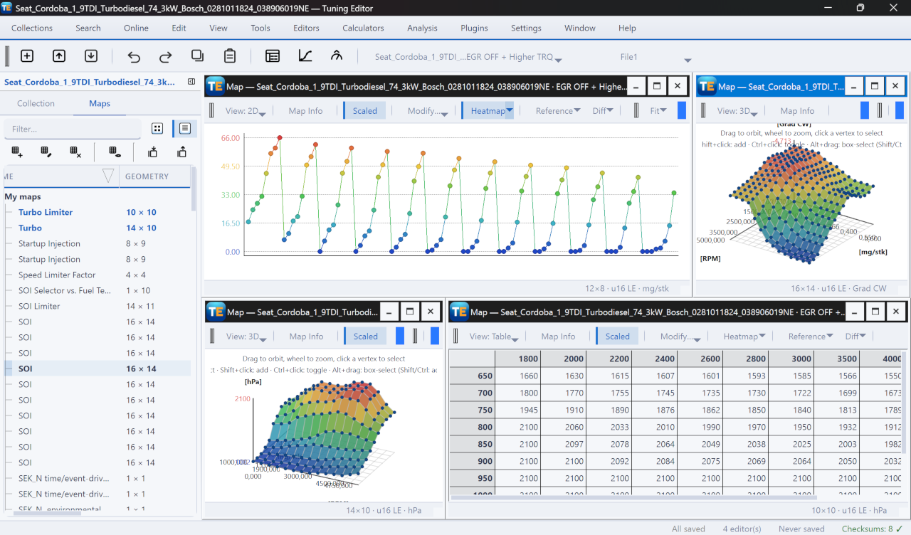
A free, modern Windows software for viewing and editing ECU calibration data - map and hex editors, tuning calculators, and online services.
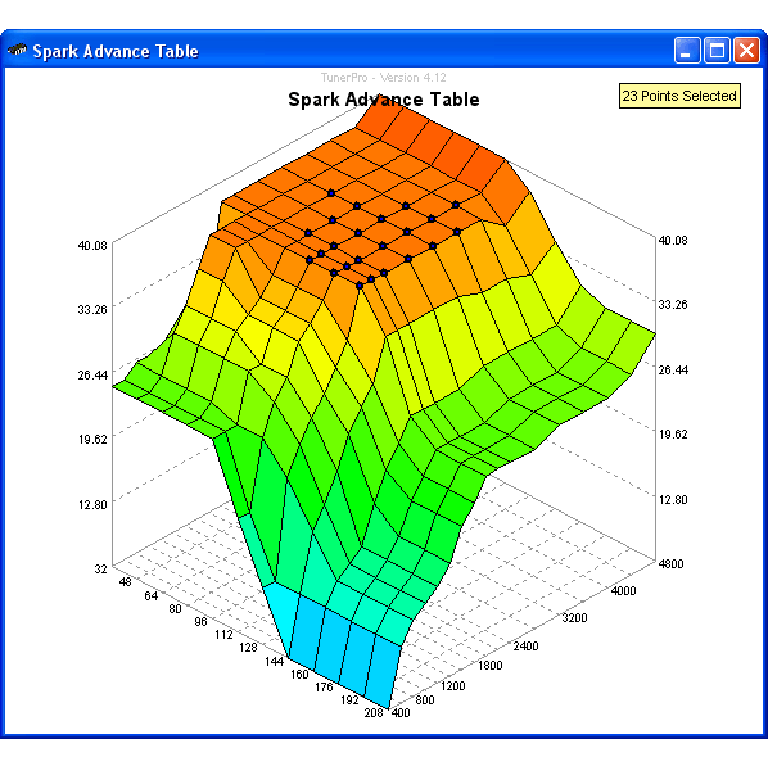
A free collection of checksum correction plugins for TunerPro that ensures safe ECU tuning. Automatically verify and update file checksums for reliable vehicle performance.